Machine Learning (ML) Concepts and in Azure

Source: My personal notes and comments from course series Introduction to AI in Azure, Introduction to Machine Learning Concepts - Training | Microsoft Learn, and training session led by Kristin Deokiesingh

Introduction

ML is like intersection of data science and software engineering with goal to create a predictive model to use in software.

Data scientists prepare data to train the model and software developers apply the model to predict new data values. The process of prediction is known as inferencing.

What is ML

ML comes from mathematics modeling and statistics with idea of using past data to predict unknown values.

For example, a doctor using clinical patient data to run automated test to predict diabetes risks for patients using weight, blood, glucose level and other measurements.

Machine Learning as a Function, Prebuilt Models use Training Data

Evaluate model; compare labels to predict y(x)
        |                         |
        |                         |
Training data --> Algorithm --> Model
        |                |
        |                |
Features (x), Label (y)  |
                         |
                         x, y relationship

Example

y = label, # of ice cream sold = f(x)
x = features, variable influencing sales, like day, season, weather, temperature
- Can be a vector = [x1, x2, x3, …]
Algorithm - find relationships between features and the label and generalize to a calculation

An ML model is software that encapsulates a function to calculate an output value y = f(x) using input values x

When training is completed, the model is used for inferencing and wrapped inside software. Users can input x values to get a y output. Sometimes output from the function shown as ŷ (called “y-hat”) to indicate it is a calculated prediction and not an observed value like the original training data labels.

Type of Machine Learning (ML), Options

Machine Learning
├── Supervised Machine Learning
│   ├── Regression
│   │   └── (Examples: temperatuve > number 5, ice cream cones)
│   └── Classification
│       ├── Binary Classification
│       │   └── (Examples: body condition > patient disease risk)
│       └── Multiclass Classification
│           └── (Examples: height > penguin type)
│
├── Unsupervised Machine Learning
    └── Clustering
        └── (Examples: plants in different clusters)

Data Format:
- Supervised Machine Learning: [x1, x2, x3], y
- Unsupervised Machine Learning: [x1, x2, x3]

Supervised Learning ([x1, x2, x3], y): Data has features and labels
- Regression: Label is numeric; Example: ice cream by season
- Classification: Label is category (class)
  - Binary - label is whether observation is or isn’t an instance of a class: patient at risk of diabetes
  - Multiclass - predict a label that represents one of multiple possible classes: species of penguin based on height
    - Models be trained to predict mutually exclusive labels. However, some algorithms can train multiple classification, allowing more than one label for an observation, like a movie categorized as sci-fi and comedy
Unsupervised Learning ([x1, x2, x3]): Training data is unlabeled, try to find similarities in observations based on features and group them into cluster
- Clustering: find similarities by characteristics like in plants based on size, number of leaves, petals
  - Similar to multiclass classification by categorizing observations into groups. Difference is categories are known with supervised learning with multiclass and unsupervised learning grouping is only on similarity of features
  - Can be used to identify classes, then train a classification model, for example finding customers with similarities, then segmenting them on features with labels to predict categories of new customers

Regression

Model creation is iterative and models are refined by repeating training with different algorithms and parameters until an acceptable level of prediction accuracy.

4 Elements of Training Process

1 Training data / Split –> 2 Algorithm –> 3 Predictions y = f(x) –> Compare to observed data labels

Split the training data randomly. One subset is used for training data. Other subset will be uses for model validation.
Algorithm, in the case of regression model, use a regression algorithms like linear regression
Use validation data subset to test the model by predicting labels
Compare to the actual labels from the validation data. Aggregate the differences between predicted and actual label values to calculate a metric showing the prediction accuracy.

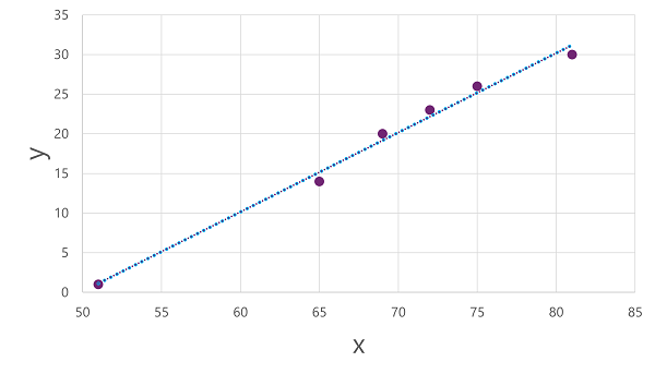
Example - Regression

Data is Features: Temperature (x) to Label: Ice cream sales (y). In practice, there are multiple features in a vector. This example simplifies to 1 feature.
Split the data randomly, so subset of Temperature to Ice cream sales is selected
Plot a graph of temperature against ice cream sales and find an algorithm the approximates y given x. An example is linear regression which derives a functions that products a straight line through observed intersections of x and y which minimizing the average distance between the line and observed points.
Evaluate the function. Using data, a possible function is f(x) = x-50. Use the validation data set feature x values and apply the function to check how close the model output is to the actual labels.

Source:

+--------------------------------------------------+
|                                                  |
| 35 +                                             |
|    |
|    |
| 30 +                        *
|    |                       /
|    |                      /
| 25 +                     *
|    |                    /
|    |                   /
| 20 +                  *
|    |                 /
|    |                /
| 15 +               *
|    |              /
|    |             /
| 10 +            *
|    |           /
|    |          /
||5+         */
||   \       /*
||   \     /*
||0+*----/----------------------------------------+
50   55   60   65   70   75   80

Regression Evaluation Metrics

Common metrics used to evaluate the regression model

Mean Absolute Error (MAE)

Checks size of errors in predictions. It doesn’t matter if the prediction was over or under (for example, -3 and +3 both indicate a variance of 3). The metric is known as the absolute error for each prediction, and can be summarized for the whole validation set as the mean absolute error (MAE).

In the ice cream example, the mean (average) of the absolute errors (2, 3, 3, 1, 2, and 3) is (2 + 3 + 3 + 1 + 2 + 3)/6 = 2.33 which is sum of values / number of the values
Mean Squared Error (MSE)

Takes all discrepancies between predicted and actual labels into account equally. It can be desirable to have a model that is consistently wrong by a small amount than one that makes fewer, but larger errors.

A method to create a metric that “amplifies” larger errors is by squaring the individual errors and calculating the mean of the squared values.

In our ice cream example, the mean of the squared absolute values (which are 4, 9, 9, 1, 4, and 9) is 6. It similar the MAE except all error variances are squared (multiplied by itself) before calculating the mean.
Root Mean Squared Error (RMSE)

Mean squared error helps take how large the errors are into account, but because it squares the error values, the metric does not represents the quantity measured by the label.

In the example, 6 is just a numeric score that indicates the level of error in the validation predictions.

To measure the error in terms of the number of ice creams and not just a score, we need to calculate the square root of the MSE, creating a metric called Root Mean Squared Error. In this case √6 is 2.45 (ice creams).
Coefficient of determination (R²)

All of metrics so far compare the variance between the predicted and actual values. In reality, there is natural random variance in daily sales of ice cream that the model takes into account.

In a linear regression model, the training algorithm fits a straight line that minimizes the mean variance between the function and the known label values.

The coefficient of determination (more commonly referred to as R² or R-Squared) is a metric that measures the proportion of variance in the validation results that can be explained by the model, as opposed to some odd aspect of the validation data (for example, a day with a highly unusual number of ice creams sales because of a local festival).

R2 is more complex then previous options and compares the sum of squared differences between predicted and actual labels with the sum of squared differences between the actual label values and the mean of actual label values, like this:

R2 = 1- ∑(y-ŷ)² ÷ ∑(y-ȳ)²

The result is a value between 0 and 1 that describes the proportion of variance explained by the model:
- Closer to 1 this value is, means the better the model fits validation data
- In example ice cream regression model, the R2 calculated from the validation data is 0.95.
Iterative Training

In most situations, data scientists need to iterate and repeatedly train and evaluate a model by changing:
- Training data used, which features, preparing data
- Algorithm selection, for example linear or other types of regression
- Algorithm parameters, accurately called hyperparameters that are separate from x and y
Iterations will use an evaluation metric and choose an acceptable model for the use case.

Binary Classification

Algorithms predict one of two possible labels like predicting true or false given features.

Example - binary classification

Look at blood glucose level x of a patient to predict if they have diabetes label y.

Training a binary classification model

Algorithm should fit training data to a function calculating the probability between 0.0 and 1.0 of the class label being true and that a patient has diabetes. For example, probability of 0.7 having diabetes compared to probability of 0.3 that the patient does not have diabetes.

In the example, logistic regression is used for classification. It is not used for regression despite the name. The keyword is logistic which describes the nature of the function (an S shaped curve) between low and high values of 0 and 1 in binary classification.

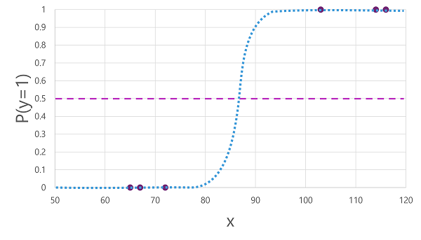
S curve on a graph. Logistic regression plot showing a sigmoid curve (blue dotted line) modeling the probability of y = 1 as a function of X. Purple points represent observed data, and the magenta dashed line at P(y=1) = 0.5 indicates the decision threshold.

1.0 |                                                                                  *****
    |                                                                              ***
0.9 |                                                                           **
    |                                                                         **
0.8 |                                                                       **
    |                                                                     **
0.7 |                                                                   **
    |                                                                 **
0.6 |                                                               **
    |                                                             **
0.5 |-----------------------------------------------------------**-------------------------
    |                                                         **
0.4 |                                                       **
    |                                                     **
0.3 |                                                   **
    |                                                 **
0.2 |                                               **
    |                                             **
0.1 |                                           ***
    |                                     ********
    +----------------------------------------------------------------
      X   50    60    70    80    90    100   110   120

The graph shows 3 points as 0 and 3 point as 1. The S curve intersects all points.

f(x) = P(y=1 | x) where it is probability of y being true (y=1) given x.

A threshold exists at the midpoint of the S curve of P(y) = 0.5. For values above it, the model predicts true and values below the model predicts false.

Evaluating a binary classification model

Like regression model training, a random subset of data is used to validate the model.

Binary classification evaluation metrics

A matrix with the number of correct and incorrect predictions for each possible class label like:


	y-hat	y-hat
y	0	1
0	2	0
1	1	3

This visualization is called a confusion matrix showing prediction totals of: In the matrix, true predictions are on the diagonal line from top left to bottom right.

ŷ=0 and y=0: True negatives (TN)
ŷ=1 and y=0: False positives (FP)
ŷ=0 and y=1: False negatives (FN)
ŷ=1 and y=1: True positives (TP)

Accuracy

Using the confusion matrix, accuracy checks the proportion of predictions that the model got right.
```
= (TN + TP) / (TN + FN + FP + TP)
= (2+3) / (2+1+0+3)
= 5 / 6
= 0.83
```
An issue with just accuracy is an example if 11% of the population has diabetes and a model always predicts 0, it would have 89% accuracy even though it doesn’t really evaluate patient features.
Recall, also called true positive rate (TPR)

The metric recall measure the portion of positive cases that the model identified correctly. So, compared to the number of patient who were observed to have diabetes, how many did the model predict to have diabetes.
```
= TP / (TP + FN)
= 3 / (3 + 1)
= 0.75
```
So the example model predicted 75% of the patients who have diabetes correctly.
Precision

Similar to recall, precision looks at predicted positive cases and check where the true label is actually positive. In the example, precision looks at portion of patients predicted by the model as true and whether they actually have diabetes.
```
= TP / (TP + FP)
= 3 / (3 + 0)
= 1
```
So 100% of the patients predicted to have diabetes by the example model, have diabetes

F1-score

Combining recall and precision is a metric called F1-score.

= (2 x Precision x Recall) / (Precision + Recall)
= (2 x 1 x 0.75) / 1 + 0.75)
= 0.86

Area Under the Curve (AUC)

Another name for recall is the true positive rate (TPR) and an equivalent metric is false positive false (FPR) calculated as:

= FP / ( FP + TN ) = 0 / 2 = 0

Both TPR and FPR metrics can be used to evaluate the model by plotting a received operator characteristic (ROC) curve that compares the TPR and FPR for every possible threshold value between 0.0 and 1.0.

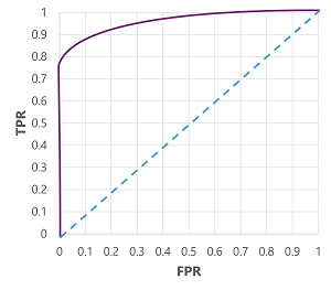
Plot of FPR vs TPR with Received operator characteristic (ROC) curve

Example possible ROC curves:
- The ROC curve for a perfect model would go straight up the TPR axis on the left and then across the FPR axis at the top. Since the plot area for the curve measures 1x1, the area under this perfect curve would be 1.0 (model is correct 100% of the time)
- A diagonal line from the bottom-left to the top-right represents the results that would be achieved by randomly guessing a binary label; producing an area under the curve of 0.5. In other words, given two possible class labels, you could reasonably expect to guess correctly 50% of the time.
In the example, the area under the curve (AUC) metric is 0.875 meaning the model performs better than random guessing (0.5).

Multiclass Classification

Multiclass predicts which of multiple possible classes a feature belongs to.

Example - multiclass classification

We have observation of penguins and their flipper length feature (x). For each observation, there is the penguin species label (y).

Training a multiclass classification model

A multiclass classification model require an algorithm to fit the training data to calculate the probability value for each possible class.

The following are kinds of algorithms.

One-vs-Rest (OvR) algorithms

OvR algorithms train a function probability prediction for each class

For the penguin example with 3 possible species, the algorithm create three binary classification functions:

f0(x) = P(y=0 | x) f1(x) = P(y=1 | x) f2(x) = P(y=2 | x)

Each algorithm produces a sigmoid function that calculates a probability value between 0.0 and 1.0. A model trained with OvR predicts the class for the function that produces the highest probability.
Multinomial algorithms

A multinomial algorithm creates a single function that returns a multi-valued output. The output is a vector (array of values) that contains the probability distribution for all possible classes - with a probability score for each class which when added up to 1.0:

f(x) =[P(y=0|x), P(y=1|x), P(y=2|x)]

An example of this kind of function is a softmax function with example output:

[0.2, 0.3, 0.5]

The elements in the vector represent the probabilities for classes 0, 1, and 2 respectively; so in this case, the class with the highest probability is 2 at 0.5.

All algorithms will use the function outputs to determine the most probably class (y) given a set of features (x).
Evaluating a multiclass classification model

Evaluation can be done by calculating classification metrics for each class or calculate aggregrate metrics that take all classes into account.

A confusion matrix can be used similar to binary classification, except the matrix shoes the number of predictions for each combination of y-hat and actual class y:

y-hat y-hat y-hat
y 0 1 2
0 2 0 0
1 1 2 0
2 0 1 2

For each class, evaluation metrics used in binary classification can be used like:

Class TP TN FP FN Accuracy Recall Precision F1-Score
0 2 5 0 0 1.0 1.0 1.0 1.0
1 2 4 1 0 0.86 1.0 0.67 0.8
2 2 4 0 1 0.86 0.67 1.0 0.8


	y-hat	y-hat	y-hat
y	0	1	2
0	2	0	0
1	1	2	0
2	0	1	2

Class	TP	TN	FP	FN	Accuracy	Recall	Precision	F1-Score
0	2	5	0	0	1.0	1.0	1.0	1.0
1	2	4	1	0	0.86	1.0	0.67	0.8
2	2	4	0	1	0.86	0.67	1.0	0.8

Clustering

Unsupervised ML uses clustering where observations are grouping into clusters based on similarities of features and where there are no known labels.

Example - clustering

A botanist observes flowers and records the number of leaves and petals on each flower. There are 2 features: leaves and petals. The goal is to group the flowers based on the features and not the identify the species, though identification could be an example of using clustering results to later build a classification model.

Training a clustering model

Algorithm: K-Means clustering
- Features (x) are vectorized to n-dimensional coordinates (n is the number of features). In the example, we use leaves (x1) and petals (x2) and would have coordinates in 2 dimensional space [x1, x2]
- The data scientist decides on the number of clusters to group the flowers - call this value k. For example, using 3 cluster, k = 3. The k points are plotted at random coordinates. These points become centre points for each cluster and are called centroids.
- Each data point (observed flower) is assign to its nearest centroid
- The centroids are moved to the centre of the data points assigned to it based on mean (average) distance between the points
- After the centroid moves, the data points are reassigned to clusters based on the new closest centroid.
- The centroid movement and cluster reassignment can be repeated until becoming stable or set number of iterations
Animation of cluster creation, centroid movement, and data point centroid reassignement

Evaluating a clustering model

With no labels to compare to, evaluation is based on how well resulting cluster are separate from one another, similar to uniqueness.

Possible metrics to check separation are:

Average distance to cluster center: How close, on average, each point in the cluster is to the centroid of the cluster.
Average distance to other center: How close, on average, each point in the cluster is to the centroid of all other clusters.
Maximum distance to cluster center: The furthest distance between a point in the cluster and its centroid.
Silhouette: A value between -1 and 1 that summarizes the ratio of distance between points in the same cluster and points in different clusters (The closer to 1, the better the cluster separation).

Deep Learning (subset of ML)

Deep learning is an advanced form of ML that tries to emulate how the humain brain learns.

Like human neural network -> Artificial neural network the simulates biological neuron electrochemical activity with math functions

Each neuron is a function of input value x and weight w
Function is wrapped in activation function to determine whether to pass output on

Neural networks are multiple layers of neurons, essentially a deeply nested function, hence the name deep learning. Models produced by it may be called deep neural networks (DNNs)

Functions in deep learning like other ML concepts predict a label (y) based on features (x). f(x) function is the outer layer of a nested function in which each layer encapsulates functions that operator on x and the weight w value associated with them. The algorithm used to train the model involves iteratively giving features (x) through the layers to calculate values for y-hat. Iterations involve validating the variance in y-hat and y values (level of error or loss in the model) and modifying weights (w) to reduce loss. The final model includes weight values that result in most accurate predictions.

Simplified neural network diagram

All neurons have connections with ones in the next layer and the are multiple layers, but not shown in detail in this diagram

            Middle layers:
            Activation Function with weights for each
            neuron to neuron connection

              O
Input Layer  /|\
            | | |              Output Layer
      O-----O-O-O-O-O-O        with softmax function
      /\    |/|\|/|\|/|\       applied for probability
      O-----O-O-O-O-O-O-O---------------O
       \    |/|\|  /|\|/|\ /
        ----O-O-O--O-OO-O---------------O
            \|/    \|/
             O      O

Example - Using deep learning for classification

Deep Learning example: A neural network processes input data through multiple layers to product accurate predictions on a penguin species based on penguin observed characteristics

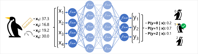
In the example explained in the image caption, feature data (x) has measurements of a penguin:

The length of the penguin’s bill.
The depth of the penguin’s bill.
The length of the penguin’s flippers.
The penguin’s weight.

x will be a vector of four values = [x1, x2, x3, x4] and y is the species of penguin like:

Adelie
Gentoo
Chinstrap

The example is a classification problem where the ML model predicts the probable class given the observations.

So y is a vector of three probability values; one for each class: [P(y=0|x), P(y=1|x), P(y=2|x)]

The process for inferencing a predicted penguin class is:

Feature vector with penguin features is fed into input layer, which consists of a neuron for each x value. Example: [37.2, 16.8, 19.2, 30.0]
First layer of neurons (functions) each calculate a weighted sum by combining the x value and w weight and pass to an activation function that determines if it meets the threshold to be passed on to the next layer.
Each neuron in a layer is connected to all of the neurons in the next layer (architecture sometimes called fully connected network). Results of each layer are fed forward through the network until they reach the output layer.
Output layer produces a vector, using a softmax or similar function to calculate the probability distribution for the three possible classes of penguin. In this example, the output vector is: [0.2, 0.7, 0.1]
The elements of the vector represent the probabilities for classes 0, 1, and 2. The second value is the highest, so the model predicts that the species of the penguin is 1 (Gentoo).

The softmax function’s use is prior to applying softmax, some results (tuple components) could be negative, or greater than one; and might not sum to 1; but after applying softmax, each component will be in the interval ( 0 , 1 ), and the components will add up to 1, so that they can be interpreted as probabilities. -Wikipedia

In the example, output vector after the softmax function shows probabilities for each penguin type of [0.2, 0.7, 0.1] instead of the output layer’s vector which can have negative and large numbers.

How does a neural network learn?

Weights are used to help calculate predicted values for labels. The model will learn the weights during training for the most accurate predictions.

The training process:

Training data is set and fed into input layer
Neurons in each layer apply weights that are randomly assigned at start
Output layer creates a vector for label predictions (y-hat)
A loss function compares y-hat to known y values and aggregates difference known as loss.
- Example, if known class is Chinstrap penguin, y value should be [0.0, 0.0, 1.0]. The absolute difference between this and the ŷ vector is [0.3, 0.1, 0.4].
- The actual loss function calculates the aggregate variance for multiple cases and summarizes it as a single loss value
The network is a large nested function and an optimization function can use differential calculus to check the influence of each weight on the loss. Then weights can be adjusted up or down to reduce loss. Optimization techniques vary, but usually a gradient descent approach where weights are set up or down to minimize loss.
Process is repeated, with iterations called epochs, until loss is minimized.

Vector Calculations and Computer Hardware used in Model Training

Conceptually, training data for each can goes through the network one at a time. In reality, data is batched into matrices and processed using linear algebra.

As a result, neural network training is best performed on computers with graphical processing units (GPUs) that are optimized for vector and matrix manipulation.

Transformers

Transformers and Language Models

Current generative AI applications use transformer architecture which improve models’ ability to understand and generate text. The method is build on success in modeling vocabularies to support NLP tasks and generating language.

Transformer architecture as two components:

Encoder block: processing input and create a representation with context of tokens, creates semantic representation of the training vocabulary
Decoder block: generates new language sequences, generative output by looking at the encoder’s representation and predicting the next token in the sequence
Transformer models - trained on large text data to understand semantic relationships to determine probable sequences of text
- Two blocks:
  - Encode block - creates relationships of training data
    - Example: BERT used in Google search
  - Decoder block - generate new content
    - Example: GPT
- Each text data is tokenized:

With training, many tokens are compiled.

+------------------+
|   1.Input Data   |
|   (Documents)    |
+------------------+
          |
          v
---------------------------------------------
+------------------+                        |
|   2. Encoder     |               Model    |
|                  |                        |
+------------------+                        |
          |                                 |
          v                                 |
+-----------------------+                   |
|  3. Collection        |                   |
|-----------------------|                   |
| dog:      [10,3,2]    |                   |
| cat:      [10,3,1]    |                   |
| puppy:    [52,1]      |                   |
| skateboard: [-3,-3,2] |                   |
+-----------------------+                   |
          |                                 |
          v                                 |
+------------------+                        |
|   4. Decoder     |                        |
|                  |                        |
+------------------+                        |
--------------------------------------------|
              ^         |
              |         |
              |         |
+-------------|----+    |
|  5. Output  |    |    |
| "When my dog was |    |
|                  |    |
|  ... a puppy" <-------|
+------------------+

Model is trained with large amount of natural language text often from internet and public text.
Sequences of text are broken down into tokens and encoder block process them using a technique called attention to determine relationships between tokens like which tokens are related to presence of other tokens in a sequence.
Collection of vectors that represents semantic attribute of the tokens. Vectors are called embeddings.
The decoder block looks at a new sequence of tokens and uses embeddings generate a natural language output.
Example: with input sequence like “When my dog was” the model can use the attention technique to analyze the input tokens and the semantic attributes encoded in the embeddings to predict completion of the sentence, such as “a puppy”.

Example implementations:

Bidirectional Encoder Representations from Transformers (BERT) model by Google to support search engine uses only the encoder block, while the
Generative Pretrained Transformer (GPT) model by OpenAI uses only the decoder block

Tokenization and Embeddings

See Tokenization and Transformers section of Microsoft Azure AI Fundamentals, Generative AI - Microsoft Azure AI Fundamentals: Generative AI
Positional Encoding

Transformers use positional encoding which is the sum of word embedding vectors and positional vectors. The result is encoded text has information about the meaning and position of a word in a sentence.

To encode the position of a word in a sentence, a single number represents the index value.
Attention and Relationships

Attention is used to establish relationship between tokens. Self-attention involves considering how other tokens around one particular token influence that token’s meaning

Encoder and decoder blocks in a transformer model include many layers of the neural network. One of the types of layers are attention layers.
- Encoder block: each token is examined in context and encoding determined for its vector embedding. Vector values are based on relationship between token and other tokens it frequently appears with. Context is taken so the same word may have multiple embedding values depending on context. Example “the bark of a tree” and “I heard a dog bark”.
- Decoder block: attention layers help predict the next token in sequence. For each token generated, the model has an attention layer taking into account the sequence of token at that time and look at which tokens are most important. Example: For “I heard a dog bark”, the attention layer may assign higher weight to “heard” and “dog” when generating the next work in sequence.
- Positional encoding layer adds a value to each embedding to indicate its position in sequence:
```
[1,5,6,2] (I)
[2,9,3,1] (heard)
[3,1,1,2] (a)
[4,10,3,2] (dog)
```
- Attention layer: deals with vectors of tokens, not the actual words. It assigns numeric weight to each token in the sequence. Calculation is done on the weighted vectors to create an attention score to help with prediction.
  - The attention function calculations help determine the most relevant output. Transformers use multi-head attention meaning tokens are processing by the attention function in parallel to get different kinds of information from a sentence.
  - The neural network evaluates all possible tokens to determine the most probable token. This process continues for each token with each input used regressively as input for the next iteration.
Transformers use an attention function where a new word is encoded using positional encoding and represented as a query. The output of encoded word is a key with a related value. For example, Vincent Van Gogh is a query and related to the key painter. The key and values are stored in a table for decoding later.
Simplified Representation of the Process
1. Token embeddings are fed into the attention layer
2. Decoder predicts the next token in the sequence, a vector in line with an embedding in the model’s vocabulary.
3. Attention layer evaluates the sequence so far and assigns weights to each token to represent their relative influence on the next token.
4. Weights help compute a new vector for the next token with an attention score. Multi-head attention uses different elements in the embeddings to calculate multiple alternative tokens.
5. Neural network uses scores in the vectors to predict the most probable token from the entire vocabulary.
6. The predicted output is added to the sequence and used as the input for the next iteration.
Model Training

During training, the actual sequence of tokens is known and later ones are masked for validation. As in any neural network, the predicted value for the token vector is compared to the actual value of the next vector in the sequence, and the loss is calculated. The weights are then incrementally adjusted to reduce the loss and improve the model. When inferencing (predicting a new sequence of tokens), the attention layer applies weights to predict the most probable token in the model’s vocabulary that is semantically aligned to the sequence so far.

Example: a transformer model like GPT-4 (the model behind ChatGPT and Bing) is designed to take text input (called a prompt) and generate a syntactically correct output (called a completion). The model uses its large vocabulary and the ability to generate meaningful sequences of words. The model relies on its training of large volume of data (public and licensed data from the Internet) and complexity of the network.

More about Models, Transformer Architecture

Read more about Transformer model based on encoder, decoder in Attention is All You Need paper

Encoder Model

Converts input to machine-readable tokens
Use case: understanding model

Decoder Model

Takes input and translates to machine-readable format
Tries to predict next output
Use case: generative model

Transformer Model

Uses encoder for understanding
Uses decoder for generation

Language Models

Data -> Encoder -> Transformer Model (Vector DB) uses embeddings
                        |
                        |-> Decoder -> Output

Tokenisation - transforms sentence words to numbers, a mathematical translation of words to tokens; 1 token is about 4 characters

Language Models and Attention

Captures strength of relationships between tokens using attention technique

Example: “I heard a dog _”
- Predict word after “dog”
- “heard” and “dog” have more weight
- Most probable token added: “bark”
Fine-Tuning Models means customizing a model for specific tasks

Machine Learning in Azure

Section looks at how to design a ML solution with Microsoft Azure using 6 steps:

Define problem and decide on type of model
Get data
Prepare data - explore, clean, and transform data for the model
Train model - choose algorithm, hyperparameter values and experiment.
Integrate the model - deploy to an endpoint
Monitor - check the model’s performance

Models can be used in Azure Machine Learning as well as be exported for outside use.

Define the Problem (Use Case)

Determine the model’s output, type of ML task, and success criteria.

Common ML tasks are:

Classification: Predict a categorical value.
Regression: Predict a numerical value.
Time-series forecasting: Predict future numerical values based on time-series data.
Computer vision: Classify images or detect objects in images
Natural language processing (NLP): Extract insights from text.

Example

Determining if patients have diabetes.
- Data: patient health
- ML tasks: Classification with category of yes or no for diabetes
ML Steps
- Load data: Import and inspect the dataset.
- Preprocess data: Normalize and clean for consistency.
- Split data: Separate into training and test sets.
- Choose model: Select and configure an algorithm.
- Train model: Learn patterns from the training data.
- Score model: Generate predictions on test data.
- Evaluate: Calculate performance metrics.
Get and prepare data

Identify data source and formats, how to provide the data, and design data ingestion. Example is data source is a CRM system in a SQL database which uses a tabular data format that is structured.

A data ingestion solution might be Extract, Transform, and Load (ETL) or Extract, Load, and Transform (ELT) where a service provides data for ML model training. A data ingestion pipeline is a set of tasks that processes the data for the model.

Example pipeline:
- Get raw data from data source
- ETL with Azure Synapse Analytics or Databricks
- Store prepared data in Azure blob storage
- Train model with Azure Machine Learning
Example implementation:

json > table > transform data
Train the Model

Considerations:
- Type of model
- Control over training
- Time/budget available
- Services, knowledge in organization, including preferred programming languages
Azure services for training ML models:
- Azure Machine Learning to train and manage your machine learning models. Studio for UI or use Python SDK or CLI
- Azure Databricks is a data analytics platform for data engineering and data science. It uses Spark compute process data. Azure Databricks can both train and manage models or integrate with Azure ML
- Microsoft Fabric is an integrated analytics platform for data workflows between data analysts, data engineers, and data scientists. It is a tool to prepare data, train a model, use the trained model to generate predictions, and visualize the data in Power BI reports.
- Azure AI Services is a collection of prebuilt machine learning models you can use for ML tasks. The models are offered as an application programming interface (API). Some models can be customized with your own training data
1. Azure Machine Learning
  
  Supports:
  - Data preparation
  - Training and evaluating machine learning models
  - Registering and managing trained models
  - Deploying models for use
  - Applying responsible AI
  It takes care of:
  - Storage and management of data for model training and evaluation
  - Automated ML (AutoML) allowing multiple training jobs (algorithms, parameters) to find the best model
  - Pipelines for training and inferencing
  - Integration with ML frameworks like MLflow
  - Metric visualization and evaluation, like check against responsible AI fairness and others
  - Compute needed for tasks described
2. Use Azure Machine Learning studio
  
  A browser portal for Azure Machine Learning studio allows using Azure Machine Learning. Get started with an Azure Machine Learning workspace which will work with other Azure resources like storage accounts and VMs.
  
  The studio allows data model, and compute management, notebook coding, pipelines, AutoML, deployment, and importing models.
  
  Available compute are:
  - Central Processing Unit (CPU) or a Graphics Processing Unit (GPU) - For smaller tabular datasets, a CPU is sufficient and cost-effective. For unstructured data like images or text, GPUs are more powerful and efficient. GPUs can also be used for larger tabular datasets, if CPU compute is proving to be insufficient.
  - General purpose or memory optimized - Use general purpose to have a balanced CPU-to-memory ratio, which is ideal for testing and development with smaller datasets. Use memory optimized to have a high memory-to-CPU ratio. Great for in-memory analytics, which is ideal when you have larger datasets or when you’re working in notebooks.
  Azure Automated Machine Learning will automate assignment of compute and iterative tasks of model development.
3. Integrate a model - Deployment and Application Use
  
  Models are deployed to endpoints. An endpoint is a web address applications can call for responses.
  1. Real time and Batch
    - Real time predictions - good for apps or websites needing immediate feedback like a retail store
    - Batch predictions - good for reports, where data can be submitted for processing later
    Consider requirements for frequency of predictions needs, compute, and individual vs batch data input. For example, if model predictions are only needed at certain times, batch predictions work.
  2. Compute
    
    Real time prediction may need container services like Azure container instance (ACI) and Kubernetes.
    
    For batch predictions, they might be done in parallel or large workload in a cluster which can be turned off after, saving costs.

Explore Automated Machine Learning in Azure Machine Learning - Demonstration in Azure

Use the Azure ML Studio to create a workspace

Choose: Data -> Choose algorithm -> Output model

Data could be in a website, cloud storage